ICFP Contest 2024 Write-up By Team powder

Created: July 3, 2024.

The International Conference on Functional Programming holds an annual programming contest to attract attention to applications of functional programming. This isn’t your average competitive programming contest. The problems are usually designed in some way around functional programming and programming language theory concepts, rather than raw number crunching. More often than not, they are also NP-complete (or worse), and it isn’t expected that anyone comes up with a perfect solution. A typical approach involves some amalgamation of slow exact algorithms, fast approximate algorithms, and even solutions by hand. It is a 72-hour marathon of coming up with the best heuristics to an unsolvable problem.

I participated in the contest in a 2-person team (powder: @mniip, @savask), using primarily Haskell. Here’s how it went.

This year the contestants were given a “communication channel” to a mysterious system (School of the Bound Variable), which accepts and returns encoded expressions in a simple lambda-calculus-based language with the following grammar (called ICFP expressions):

data Expr = EBool Bool | EInt Natural | EText Text -- data
  | EUnary UnaryOp Expr | EBinary BinaryOp Expr Expr -- operations
  | EIf Expr Expr Expr
  | ELambda Natural Expr | EVar Natural -- lambda calculus (see Apply below)

data UnaryOp = Negate | Not | EncodeBase94 | DecodeBase94

data BinaryOp = Add | Sub | Mul | Quot | Rem -- EInt operations
  | Less | Greater | Equal -- comparison
  | Or | And -- EBool operations
  | Concat | Take | Drop -- EString operations
  | Apply -- Apply lambda function to argument

The mysterious system uses a wacky character encoding with only 94 characters for its strings, and EncodeBase94/DecodeBase94 convert between strings and natural numbers using base-94.

Hello

Learning to communicate with this server earns the team points for the hello task. E.g. sending the string "get index" (encoded as S'%4}).$%8) would return a text document containing an index page with pointers to other places of interest. Initially the server would simply return a string literal (an EText expression), but sometimes it would return unevaluated programs and we have to evaluate them. This culminates in the “language test”, a program sent by the server that validates each operation in the ICFP expression language, and if successful, gives you a magic incantation that you can send to the server to score points for it.

We implemented a very naive big-step term rewriting evaluator. The task prescribes call-by-name (not call-by-need, no thunks!) and we did just that, and that was mostly enough until the end of the contest.

LambdaMan

Digging deeper into the server we discover a task description for what amounts to the following problem: given a maze on a rectangular grid, you have to give a sequence of directions that visits every free cell at least once. Your score is the size of your input (lower is better).

Not the length of the sequence of directions, but rather the length of the ICFP expression you send to the server. That means for repetitive strings it’s better to send a program that evaluates to the needed string, instead of just the string literal itself.

At this point we figured we’ll be needing to write a lot of programs in this language, so we implemented a translator from Haskell syntax to this language. Most of the work is done by template-haskell (Haskell’s proc macro system), and all we have to do is map the Haskell AST constructs to ICFP expressions. Notably, every single lambda and variable counts, so we don’t do any desugaring that hides code size.

Finding the shortest program that outputs a given string is an instance of Kolmogorov complexity, which is actually equivalent to the halting problem, so no perfect solution is possible.

For any maze we can generate a string that solves it and then compress it, although generating the shortest string is not that easy, and I conjectured that it’s NP-complete. For compression, we’ve tried a combination of run-length-encoding, common substring elimination, and conversion to base-4. A couple mazes can be solved by always repeating every step twice, which further halves the size of the base-4 encoding.

template-haskell allows some slick staged metaprogramming here, and our code looked something like this:

lambdaman5 = $(lift . fromHaskell =<< [|
    "solve lambdaman5 " <>
    let go = $(baseDecoder "UDLR")
    in go go $(lift $ encodeBase "UDLR" "RDLLLULU[...]UULULLLL")
  |])

This alternates execution of actual Haskell code (encodeBase), and Haskell syntax that is merely translated into ICFP expressions (let go =), and ultimately produces this submission:

"solve lambdaman5 " <> let
    x0 = \x1 x0 -> if x1 == 0
      then ""
      else take 1 (drop (x1 `rem` 4) "UDLR") <> x0 x0 (x1 `quot` 4)
  in x0 x0 11246230[...]19159975

On the other hand, for more regular-looking mazes we can manually come up with a short and hand-optimized program that generates a solution according to a particular pattern. For example, this is a very compact program that sweeps out a 27x27 rectangle:

let
  thrice x = x <> x <> x
  times27 x = thrice (thrice (thrice x))
in times27 (times27 "R" <> "D" <> times27 "L")

Of note is that direction commands that would run you into a wall are simply ignored, and your program can output a lot of these “waste” commands if it helps keep the program short. times27 made a frequent appearance because its code is just so short, even if we only needed to repeat something like 4 times.

At some point we discussed the idea of outputting random walks, but quickly dismissed it because we thought it would be unlikely that a random walk could actually fill the entire maze given a reasonable amount of steps. Turns out many other teams successfully employed this very strategy!

Spaceship

Another available task was to control an inertial spaceship to make it visit a given set of points on a plane.

The input is a sequence of accelerations at each time step. The spaceship is capable of accelerating by -1, 0, or +1 in both the X and Y directions. At each time step, this acceleration is first added to its velocity, and then the resulting velocity is added to the position. A point counts as visited if the spaceship was at that point at the end of the time step. The score is the number of time steps taken (no program compression shenanigans this time).

A lot about the spaceship’s motion can actually be expressed analytically, and this opens the door to a rather efficient approach to the problem.

Reducing the problem to 1 dimension, if the spaceship is moving at constant acceleration $a$, starting from velocity $v_0$ and position $x_0$, then at time $t$ its position becomes:

\[x = a\frac{t(t+1)}{2} + v_0t + x_0\]

The deviation from the standard parabolic motion equation is due to the discretization of time.

If the acceleration is not constant, then the velocity always changes by the sum of the accelerations, independent of the order of the commands. However the change in the position does depend on the relative order of the commands.

A key observation here is if that we put a bunch of -1’s first, and then a bunch of +1’s, then that would correspond to the most negative change in position, for a given change in velocity, and given duration. Likewise, putting all +1’s first, and all -1’s after, corresponds to the most positive change in position for a given change in velocity and given duration. These represent two extremal “strategies” of changing your velocity.

A second key observation is that every intermediate change in position is attainable by some intermediate strategy. The set $S(t, v_0, v_1)$ of positions attainable in $t$ steps while also changing your velocity from $v_0$ to $v_1$ is the union of the three sets

\[S(t, v_0, v_1) = \bigcup_{a \in \{-1, 0, +1\}} S(t - 1, v_0, v_1 - a) + v_1\]

where $a$ is the acceleration you use at the last step. The extremal strategies line up so that these three sets always overlap, and by induction on $t$ we conclude that $S(t, v_0, v_1)$ is always a consecutive range.

Thus the inequalities for the two extremal strategies act as an analytical expression of when a specific maneuver is possible:

\[t^2 + 2t(v_1 + v_0) - (v_1 - v_0)^2 + 2(v_1 - v_0) - 4(x_1 - x_0) \ge 0\] \[t^2 - 2t(v_1 + v_0) - (v_1 - v_0)^2 - 2(v_1 - v_0) + 4(x_1 - x_0) \ge 0\]

We constructed these as conditions on $x_1$, but we can just as well use them as conditions on $t$ given $v_0, x_0, x_1, v_1$. From the fact that these are quadratic inequalities and that $t$ must be non-negative, we can conclude that the set of solutions for $t$ is the union of a ray and at most one range, and we can cheaply and exactly compute the endpoints of these rays/ranges from roots of the quadratics.

Going back to 2 dimensions, we have restrictions on $t$ from the X coordinate, and also restrictions on $t$ from the Y coordinate. These can be intersected analytically to give us a cheap algorithm to compute the smallest possible $t$ necessary to go from phase state $(x_0, y_0, v_{x0}, v_{y0})$ to phase state $(x_1, y_1, v_{x1}, v_{y1})$.

We can also analytically minimize the quadratics along the $v_1$ variable, and repeat the same process to get an algorithm that computes the smallest duration necessary to go to a specific point regardless of the exit velocity.

Once we know that a specific maneuver is possible within some time, it’s easy to reconstruct the accelerations necessary to actually perform it. That means there’s two things left to this problem: figuring out an order for visiting the points, and figuring out what velocity we’ll have at each point, both so as to minimize the sum of maneuver durations (which is cheap to calculate).

At first we focused solely on the order, leaving the velocities to a greedy algorithm. Here’s a couple typical inputs for the spaceship problem:

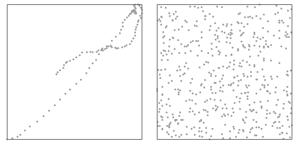
On the left, a collection of points arranged along a self-intersecting curve. On the right, a collection of points scattered completely randomly and uniformly in a square.

For the left case, the “intended” route is rather obvious, perhaps modulo choosing which branch to follow near a self-intersection. For the right case, not so much. This problem seems actually fairly similar to the Traveling Salesman Problem, but with one small twist.

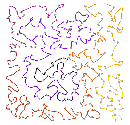
First we wrote an implementation of simulated annealing to solve TSP. We would generate random ranges of indexes to reverse, which is equivalent to picking a random pair of edges and reconfiguring them from an “X” to a “) (”, or vice versa – and then see how much the score improved or worsened. Simulated annealing would generate routes like this (shown with the maneuvers taken by the spaceship):

An untangled curve visiting points uniformly spread across a square

The twist is that using distance as a metric generates a lot of sharp turns that the spaceship has great trouble traversing because it has inertial movement. What we really want to optimize is not the distance (change in position), but change in velocity. Much like optimizing distance makes each 2-point route a straight line segment, we want to make each 3-point route a parabola. The end metric we arrived at is to minimize, for each three consecutive points $(x_0, y_0)$, $(x_1, y_1)$, $(x_2, y_2)$, the value:

\[\max(\left\vert x_0 - 2x_1 + x_2 \right\vert, \left\vert y_0 - 2y_1 + y_2 \right\vert)\]

This counts the minimal acceleration required to traverse these 3 points in sequence. We can then generate routes like this:

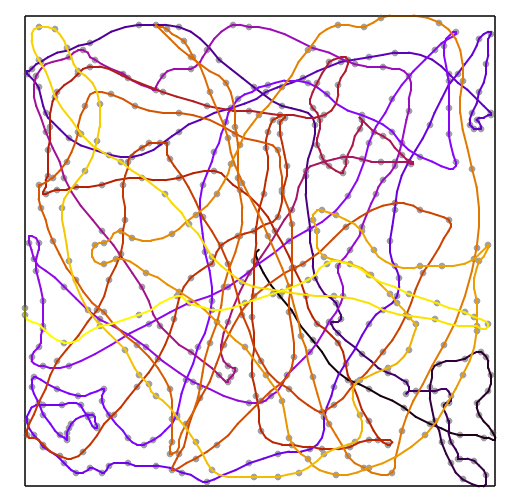
A tangled curve that is much more smooth, visiting points uniformly spread across a square

It looks much more convoluted, but actually wins 7% in terms of the final score.

After fixing a route, we can similarly use simulated annealing to pick velocities to use at each point, this time minimizing the actual resulting score – sum of times necessary for the maneuvers. Here though we have to be careful about what we consider to be neighboring states. In some cases, the space of maneuvers might be discontinuous, and not at all due to the discretization. When $x_1 - x_0 \lessapprox v_0^2/4$, it means that you’re moving too fast to gently stop at the point $x_1$, and you have to either go through it, or turn around and go back to it.

Later we also tried writing an annealer that tries to shuffle both simultaneously – the route and the velocities. That didn’t bring much profit.

Unfortunately we didn’t come up with any clever algorithm to reliably detect the order of points in the inputs that were stretched out in a curve, so we resorted to also using simulated annealing for those, which struggled at larger inputs.

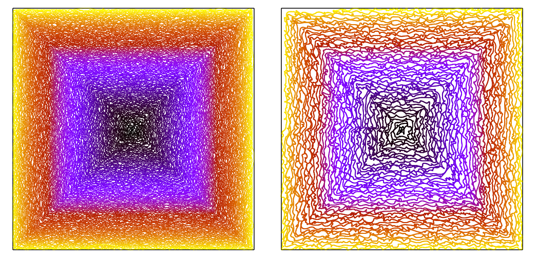
Struggling at large inputs is also why we couldn’t come up with a route for the last (25th) input. In the end we simply manually ordered the points in a thick square spiral around the center, and let maneuver annealing do the rest (right side is the center zoomed in):

On a cool but useless aside, the first solutions we had for the 24th and 25th inputs were so large they did not fit in the 1MB submission limit, and I’ve wasted a bit of time on trying to compress them (by making a program that fits within 1MB and evaluates to the submission). Simple base-9 (not 4 this time) encoding didn’t work because the decoder was actually hitting a time limit due to the quadratic complexity of the arithmetic operations it had to perform to unpack. Instead I tried to make good use of declaring common substrings as variables and then using concatenation. In the end I managed to fit a 2.9MB solution in a 0.8MB program. This proved to be useless because in the end we had solutions for these inputs that fit under 1MB.

Efficiency

We tackled the 5th available task (efficiency) before we did the 4th (3d). To even access the task we had to “exploit” a “backdoor”: one of the inputs for spaceship was actually encoded as a program that outputs the string, and in the unevaluated program there was an unused string literal containing "/etc/passwd". Following the lead, we were able to find out the Headmaster’s password by cracking its MD5 hash (luckily the password was so common the hash could simply be googled). This was one of the three ways to unlock this task, the other two being solving a few 3d problems, or waiting until the end of the lightning round of the contest (first 24 hours).

The task itself consists of 25 programs the server sends you, which you have to evaluate. We quickly found that our evaluator is not fast enough to handle these programs. I thought of reusing a cool trick that helped us win the 2020 lightning division: much like we can translate Haskell syntax into ICFP expressions, we can translate ICFP expressions into Haskell, and compile them using GHC. Very curiously, these programs actually interact uniquely poorly with the GHC simplifier, causing it to run out of memory and stack space!

While I was battling these problems, my teammate started reverse engineering the programs and discovered the true nature of the issue. These programs cannot be run on modern computers! (maybe except a couple)

For example, here’s the 4th program:

(\x1 -> (\x2 -> x1 (x2 x2)) (\x2 -> x1 (x2 x2)))
(\x4 x3 -> if x4 < 2 then 1 else x3 (x4 - 1) + x3 (x4 - 2)) 40

Recognizing the Y combinator used for recursion, we can rewrite the program as follows:

let
  x3 x4 = if x4 < 2
    then 1
    else x3 (x4 - 1) + x3 (x4 - 2)
in x3 40

Clearly, x3 is simply a naive recursive implementation of Fibonacci numbers, and the program is trying to evaluate the 40th Fibonacci number.

A compiler like GHC will never guess that it should actually completely rewrite the program using memoization/dynamic programming, that job lies on us.

Some of these problems were number theory exercises, like computing Mersenne primes. Others were straight up logic puzzles. For example, the 7th program looks like this, after some desugaring:

let
  f n = let
        x1 = 0 < n `quot` 0x1 `rem` 2
        x2 = 0 < n `quot` 0x2 `rem` 2
        x3 = 0 < n `quot` 0x4 `rem` 2
        x4 = 0 < n `quot` 0x8 `rem` 2
        x5 = 0 < n `quot` 0x10 `rem` 2
        {- ... -}
        x39 = 0 < n `quot` 0x4000000000 `rem` 2
        x40 = 0 < n `quot` 0x8000000000 `rem` 2
    in if
        (not x18 || not x15) && (not x14 || not x9) &&
        (not x19 || x37 || x12) && not x39 && (not x20 || x18) &&
        (not x8 || x16 || not x24) && (not x29 || not x39) &&
        {- ... -}
        (not x16 || not x37) && (x22 || not x14) &&
        (x28 || x8 || not x29) && x1 && (not x24 || not x32) &&
        (not x2 || not x19) && (not x31 || x13 || x14)
      then n
      else f (n + 1)
in f 1

This program splits a number into 40 bits, and tests whether they satisfy a boolean CNF formula. If not, it tries with the next number, and so on, until a match is found. Of course, finding a bit pattern that satisfies a boolean formula is a well studied problem. It’s NP-complete, but SAT-solvers are off the shelf implementations of some state of the art algorithms in this area, and indeed we were able to wrangle Z3 into solving these, including outputting the lexicographically smallest solution (which is what the program is supposed to output). Alongside the CNF formulas there were also a couple Sudokus (literally), which we also solved using Z3.

3D

The task we skipped so far was called 3d. It defined an esoteric programming language, programmed on a 2-dimensional grid, which then evolves in a third dimension of time, with multiverse time travel! It’s one of those languages where you look at the spec and think: “How do you even do anything?”.

Everything on the grid is either a number or a device. You have devices to move stuff around the grid, you have devices to do simple arithmetic operations on the numbers (addition, subtraction, multiplication, quot, rem), you have devices that test for equality and inequality.

And you have a device that lets you send a cell to some specific location some specific time ago. Doing this rollbacks the execution of the program to that moment and restarts it from there.

The task was to solve a number of programming exercises in this language. Test inputs would spawn on the locations you designated as inputs, and the program would execute until a number is pushed into a cell you designated as the output. Assuming the answer is correct, your program would be scored based on the 3-dimensional bounding box of spacetime in which it fit during its execution (lower volume is better).

The first exercise was implementing a factorial function. You can use numbers traveling in literal cycles as loops, but that unrolls the entire loop in the time dimension, giving you a terrible score. Instead you want to implement loops using time travel, which if set up correctly, makes it so that your program’s time dimension is bounded from above, no matter the number of iterations of the loop.

Using time travel poses a significant challenge though: if you have some mechanism that results in time travel being triggered, the mechanism is rolled back and will trigger time travel again, unless somehow disabled. Thus it’s easy to get stuck in an unintentional time loop, and hard to make programs using time travel composable, which is necessary for writing larger and larger programs.

At some point we did implement a simulator, but we didn’t implement a grid-based editor or anything like that, resorting to constructing and laying out programs manually in a text editor.

A few ideas that we did come up with and used in our solutions:

Computing (3*x + 2) `div` (3*x + 1) tests whether x is positive, negative, or zero.
Computing (2*x + 1) `rem` 2 yields -1 for negative x, and 1 for non-negative x, as a simplified test of positivity.
More than one cell can be designated as input (the input is cloned), and as output (first one ends the program).
Sometimes a long arithmetic circuit can be divided into two, where the output of the first half sends values into the past to the second half. This slightly increases space footprint but decreases time footprint.
The solution for problem 10 (balanced parentheses and brackets) can be reused to solve problem 9 (balanced parentheses).

Closing Thoughts

The contest was great and we had lots of fun. The problems were very diverse, but not too diverse so as to be intractable by a small team.

Solving the engineering challenges of probabilistic algorithms has always been a weak point for our team, but this year I finally felt like I understood what I was doing with simulated annealing and that I was getting useful results with it.

Tooling has also been a weak point: during previous contests we always went with the path of least resistance, which is to make a bunch of CLI programs that consume text files with problems and produce more text files with solutions, and then glue everything together with bash. This approach doesn’t really scale as you start having multiple solvers for a problem, or algorithms that improve on existing solutions, and then you want to track which solution came from where, whether they have been “improved” already, and by what, etc. Likewise, probabilistic algorithms tend to need a lot of tinkering with parameters, and may need checkpoints and so on. And of course, you have to share solutions between team members.

Unfortunately this year was no different. Last year I set out to change that, so before the contest I set up a database that could be used to manage problems and solutions and so on. But we never ended up actually using this database to manage problems and solutions, perhaps because the entry bar for hooking it up to other code was too high. Maybe next year will be different.